Reserves Evaluation for Oil, Gas, Coal, and Minerals: Price, Tech, Concentration, Rate, and Economics

     Reserves evaluation is a predictive process based on the data available. With this post, I wanted to both better understand and apply reserves analysis and compare the differences between evaluating reserves of oil vs. gas vs. coal vs. minerals. I guess it's kind of an exercise in comparisons of extracting gases, liquids, and solids in various combinations and under varying conditions. Each phase has its own physical laws to follow. Reserves usually refer to remaining reserves unless they are presented as original reserves. In the U.S. the U.S. Geological Survey is staked with assessing oil & gas, coal, and mineral resources and reserves. Resources usually refer to original resource-in-place but may also refer to remaining resource-in-place. Reserves refer to recoverable resources. This is discussed later in this post.

 

Oil & Gas Reserves Evaluation

     Oil and gas reserves may be evaluated in a number of ways. They are also often dependent on factors like geology, which can vary considerably, and can define the extent of accumulations, and thus total reserves. Reservoir qualities like porosity, permeability, pressure, natural and/or induced fractures, and intra-reservoir barriers can affect reserves evaluation. The main and most accurate means of predicting reserves is the evaluation of the production of individual wells. This is done through decline curve analysis.

 

Decline Curve Analysis

     What is decline curve analysis? According to Wikipedia:

“Decline curve analysis is a means of predicting future oil well or gas well production based on past production history. Production decline curve analysis is a traditional means of identifying well production problems and predicting well performance and life based on measured oil well production.”

Decline curve analysis can also be used to geospatially map production trends perhaps as estimated ultimate recovery (EUR) or 1st month production or maybe 1st year production. Oil and gas wells typically produce their maximum output rate shortly after production begins, usually in the first year. This early high production rate is known as ‘flush production,’ initial production, or peak flow rate. Production decline is plotted logarithmically. After flush production, well production usually levels out and curves may be forecasted out to 30 years or more. There are different types of curves used to draw out the later stabilized and relatively flat production rate. The three main ones are exponential decline, hyperbolic decline, and harmonic decline, as shown below. It should be pointed out, as the 2nd graph shows, that initial or flush production is mainly not the concern of decline curves. The main concern is to predict future production. The initial production is likely to exhibit hyperbolic decline and the later production is likely to exhibit exponential decline. Thus, as the 2nd graph shows, the two are often combined in a curve.

  

     Working as a geologist I found decline curve analysis to be a useful tool and I used it a lot. It enabled better production mapping which is tied into various kinds of geological mapping to arrive at a better understanding of field size and extents and possible geological issues affecting productivity. Decline curve analysis can also be used to discover possible mechanical issues with wells, especially if production drops significantly lower than curves suggest it should. For my purposes I used Excel’s simple logarithmic plots, but more accuracy can be attained with decline curve analysis software. This software is required for determining company-level reserves. A company’s reserves can affect its valuation, its ability to borrow money, and its ability to find development partners. The 1st graph below shows some of the common features of a decline curve. The 2nd graph is an example decline curve from a well.

 

PetroWiki states the ‘Golden rule of decline curve analysis (DCA)’

“The basic assumption in this procedure is that whatever causes controlled the trend of a curve in the past will continue to govern its trend in the future in a uniform manner.”

 

Core Areas Delineation

     Oil and gas resources and reserves are often differentiated by in-place estimates and recoverability estimates. These are often highest in the richest parts of the deposits and sometimes in the areas where recoverability is highest. This is the case with shale reserves which are often continuous over a large area. The richest parts are often called ‘core areas’ and are the most desired areas to drill due to those areas having the highest profitability. Economics dictates in most cases that these will be the areas drilled first.  

 

 

Coal Reserves Evaluation

     Unlike oil & gas which are fluids, coal and mineral ores are solid (mineral brines are an exception). Fluids flow. Solids do not flow. That means coal and mineral ores are not amenable to evaluation through rate of production. Reserves are measured differently. Coal evaluation involves an estimation of its energy value, or fuel content. This is dependent on the chemical composition of the coal, specifically the carbon, hydrogen, oxygen, nitrogen, and sulfur contents. An approximation can be estimated by calculating a coal seam’s moisture, volatile matter, ash, and fixed carbon contents. An ultimate, or elemental analysis is estimated with the atomic elements listed above. The basic formula for determining the energy value of coal from Wikipedia is gieven below.

The calorific value Q of coal [kJ/kg] is the heat liberated by its complete combustion with oxygen. Q is a complex function of the elemental composition of the coal[citation needed]. Q can be determined experimentally using calorimeters. Dulong suggests the following approximate formula for Q when the oxygen content is less than 10%:

Q = 337C + 1442(H - O/8) + 93S,

where C is the mass percent of carbon, H is the mass percent of hydrogen, O is the mass percent of oxygen, and S is the mass percent of sulfur in the coal. With these constants, Q is given in kilojoules per kilogram.

     The other main factor in coal reserves evaluation is the size/geographic extent/total volume of the coal seam. Changes in chemical composition in different geographical areas and stratigraphic sections of the seam that affect energy value must also be considered.  

     Coal energy content is also measured in terms of its gross calorific value (GCV), or higher heating value (HHV). This is used by facilities that combust coal to determine parameters such as boiler efficiency, combustion values, and production costs.

     Estimated global coal reserves by country are shown below. As can be seen, the U.S. is blessed with the highest coal reserves by a pretty good margin.

     In the U.S. the USGS assesses coal resources and reserves. Their methodology is summarized below.

Phase I: Data collection

1. geologic–drill holes, measured sections, geophysical data – that show coal bed thicknesses, partings, interburden/overburden lithologies, or structure.

2. restrictions–mostly environmental and land-use restrictions.

3. societal-boundaries, property ownership, and mineral ownership.

4. coal quality–data points that provide information on coal quality parameters. (energy content)

5. coal economics–market prices and production costs/

Phase II: Data modeling

1. correlation– estimating bed sizes and lateral continuity of individual beds

2. geologic models–using available geologic data to determine if coals are produceable, both technically and economically.

3. GIS models-use GIS to map out restrictions and other barriers to production.

4. Composite model–combine geologic and GIS models to produce a composite model of the geology, restrictions, and societal features.

Phase III: Calculating resources and reserves

1. resources calculations-use composite model to: a. calculate original resources b. calculate recoverable resources (for all significant coal beds)

2. projected mine costs-estimate cost to produce.

3. cost curve graphs-combine estimated costs with market price data to generate the graphs.

4. reserves determination-interpreted from the cost curve graphs for all significant coal beds.

 

Mineral Reserves Evaluation

     Similar to gas, oil, and coal, mineral resources estimation is done through statistical means. Typically, there is geological modeling of ore bodies, then they can be quantified with statistical methods like block modeling. Block modeling utilizes common statistical algorithms such as nearest neighbor, inverse distance weighting, and kriging. These algorithms are also used in contour mapping.

 

     “The location, quantity, grade, geological characteristics and continuity of a mineral resource are known, estimated or interpreted from specific geological evidence and knowledge.”

 

     Mineral resources can be differentiated into three classes: 1) inferred mineral resources, 2) indicated mineral resources, and 3) measured mineral resources. Inferred mineral resources are based on geological evidence but limited sampling. Sources of the sampled data may be from outcrops, trenches, pits, workings and drill holes. Grade or quality is estimated. It is assumed but not verified. Indicated mineral resources are that part of a mineral resources where “quantity, grade or quality, densities, shape and physical characteristics, can be estimated with a level of confidence sufficient to allow the appropriate application of technical and economic parameters, to support mine planning and evaluation of the economic viability of the deposit.” The data is from the same sources as for inferred mineral resources but is more extensive and reliable. Measured mineral resources are those that whose parameters “are so well established that they can be estimated with confidence.”

     Mineral reserves are classified as Probable Mineral Reserves – the economically mineable parts of the indicated and measured reserves and the processing involved to get them to market, and Proven Mineral Reserves – the economically mineable parts of measured mineral resources based on feasibility studies.

 

 

 

 

Mineral Concentration is an Important Economic Factor

     Minerals are often contained within ores, which rocks as groups of minerals and mixes of different types and at different concentrations. Thus, it is the ratios of desired mineral to total ore by weight or volume that is the determining factor in mineral resource and reserves estimation. Ore grade is often determined by desired mineral concentration(s) in the ore. Another factor in determining economic recoverability is the potential of co-production of multiple minerals. These additions to the overall economic benefit of the ore can bring a marginally profitable mineral over the threshold to profitability.

     Just as oil and gas deposits have core areas and the low hanging fruit of large accumulations found and developed, so too do mineral assemblages. The core areas become those deposits with the highest mineral concentrations so that as time goes on more of those areas with lower concentrations must be mined unless new reserves are found. That does happen so all these things occur simultaneously. Mining mineral ores with lower concentrations means several things. First, it means that the economics will be less favorable than in projects with higher concentrations. Second, there will be more ore to process for a similar amount of mineral. This also means that ore waste will be increased per kg of mineral produced. This may result in higher net impacts to the environment vs. Higher concentrated deposits. This is currently happening with copper and a few other minerals and is a matter of concern for the clean energy transition which calls for quite a large amount of copper. Below is a 2016 USGS graph of historical global copper production and a forecast of global copper production to 2100.

 

Cost and Complexity of Mineral Processing

     The cost of mineral processing is always a factor in determining economically recoverability of minerals. That cost is determined by its complexity. Processing is often called refining and compared to oil refining, which cost similarly ties into oil reserves calculation. New methods of mineral processing may become cheaper per unit of mineral processed as they are implemented.

 

Oil & Gas-In-Place, or Resource-In-Place

     For oil and gas, the Original Gas-in-Place (OGIP), aka. Gas-Initially-in-Place (GIIP) is ideally to be determined for gas reserves evaluation. This can be done before or during drilling and production. The calculation requires an estimation of the available pore space in the rock and the connectivity of that pore space (permeability), and the oil and/or gas saturation, which for gas is dependent on pressure, gas charge, water saturation, and other factors. Two summarized formulas for gas-in-place are shown below:

GIIP = Gross Rock Volume * Net/Gross * Porosity * Average Initial Gas Saturation / Formation Volume Factor1

Another equation for calculating gas in place is: G = 43,560 x A x h x φ x (1 - Sw) ÷ Bg × E234

Where A = area, h = net pay, φ = porosity, Sw = water saturation, Bg = gas formation volume factor, and E = recovery efficiency.

The detailed formulas are much longer and involve several additional calculation steps to arrive at the main variables. For oil, original oil-in-place, or stock tank original oil-in-place (STOOIP) is distinguished from remaining oil-in-place, which is sometimes just called oil-in-place. A simplified STOOIP calculation formula is shown below.

 

Recoverable Reserves

     Resource estimates, including resource-in-place estimates, are not the same as reserves. Reserves must be recoverable, whether technically (with current technology), or economically. Pricing is always a factor in economic recoverability since profit is required for businesses to succeed.

 

Technically Recoverable Reserves

     Technically recoverable reserves refer to those reserves that could be developed with current technologies but may not be economically viable to do so. Cost is a barrier to development even though we know the resources are there. With new technological developments, technically recoverable reserves can be reclassified as economically recoverable reserves. That is what happened with shale gas and oil as the new technologies of high-volume hydraulic fracturing and horizontal drilling tech unlocked new supplies that became economical. The reserves are there and may someday be profitably extracted when technology improves

 

Economically Recoverable Reserves

     Economically recoverable reserves depend on technology as stated above but they also depend on commodities pricing. Prices for oil, gas, coal, and minerals fluctuate according to supply-demand dynamics. Companies selling commodities must always consider pricing to determine profitability. Fluctuation in profitability due to pricing can lead to busts and booms and supply-demand cycles that can have some predictability.

     The Society of Petroleum Engineers (SPE) recognizes three categories of reserves:

Possible Reserves

     Possible reserves are those reserves with the “odds of commercial extraction under 50-percent, but higher than 10-percent,” according to SPE.

 

Probable Reserves

     Probable reserves are “those with the likelihood of recovery for between possible and proved reserves, or over 50-percent but under 90-percent,” according to SPE.

     Both possible and probable reserves are not yet proved, so they are deemed unproven. The difference between proved and unproved reserves is the degree of certainty about whether those reserves will be developed. These designations often change with pricing. If the price of a commodity rises so too doe the likelihood of development of more resources so some possible reserves will be reclassified as probable reserves and some probable reserves will be reclassified as proved reserves.

 

Proved Reserves (Developed and Undeveloped)

     Proved, or proven reserves have “a 90-percent or above likelihood of commercial extraction,” according to SPE. Proved reserves may be developed or undeveloped. In the case of oil and gas proved developed reserves are those that are in the various stages of being produced, from new wells with flush production to old wells with steady but much lower production. Proved developed reserves are those reserves that are expected to be recovered from existing wells. Proved undeveloped are those reserves that are expected to be developed in the future with new wells, These may include deepening existing wells or some kind of enhancement like recompletion or a  ‘refrac’ of the well. The SEC requires oil and gas companies to delineate their proved developed and proved undeveloped reserves.

 

Finding Costs and Lifting Costs

     Finding costs are simply the costs to explore for, discover, and develop a resource. The Energy Information Administration (EIA) describes finding coats as follows:

“Finding costs are the average costs of adding proved reserves of oil and natural gas via exploration and development activities and the purchase of properties that might contain reserves. These costs are measured for oil and natural gas on a combined basis in dollars per boe. Ideally, finding costs would include all costs incurred (no matter when these costs were incurred or recognized on a company's books) in finding any particular proved reserves (not including the purchases of already discovered reserves). In practice, and as reported here, finding costs are actually measured as the ratio of exploration and development expenditures (including expenditures on unproved acreage but excluding expenditures on proved acreage) to proved reserve additions (excluding net purchases of proved reserves) over a specified period of time. Finding costs are generally calculated in Performance Profiles as a weighted average over a period of 3 years.”

Lifting costs are the costs to operate and maintain wells. According to the EIA:

“Lifting costs (also called production costs) are the costs to operate and maintain wells and related equipment and facilities per barrel of oil equivalent (boe) of oil and gas produced by those facilities after the hydrocarbons have been found, acquired, and developed for production. 15  Direct lifting costs are total production spending minus production taxes (and also minus royalties in foreign regions) divided by oil and natural gas production in boe. Total lifting costs are the sum of direct lifting costs and production taxes.”

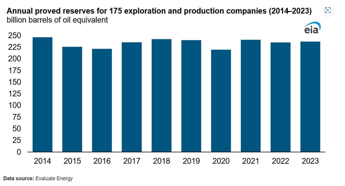
U.S. Oil and Gas Reserves and Finding Cost Changes Over the Past Decade

The graphs that follow show the changes in proved reserves and finding costs for U.S. oil and gas companies from 2014 through 2023.

 

 

References:

 

Public company proved oil and natural gas reserves were mostly unchanged in 2023. Energy Information Administration. Today in Energy. August 12, 2024. Public company proved oil and natural gas reserves were mostly unchanged in 2023 - U.S. Energy Information Administration (EIA)

Decline curve analysis. Wikipedia. Decline curve analysis - Wikipedia

Production forecasting decline curve analysis. PetroWiki. Production forecasting decline curve analysis - PetroWiki (spe.org)

What Are Decline Curves? Brookside Energy. October 2022. Oil-and-Gas-Well-Decline-Curves-Explained-v.2.pdf (brookside-energy.com.au)

5.2: Estimation of Original Gas In-Place, OGIP, Using the Volumetric Method. PNG 301. Introduction to Petroleum and Natural Gas Engineering. Penn State University College of Earth and Mineral Sciences. 5.2: Estimation of Original Gas In-Place, OGIP, Using the Volumetric Method | PNG 301: Introduction to Petroleum and Natural Gas Engineering (psu.edu)

Estimation of gross calorific value of coal: A literature review. Lethukuthula Vilakazi &Daniel Madyira. International Journal of Coal Preparation and Utilization. April 14, 2024. Full article: Estimation of gross calorific value of coal: A literature review (tandfonline.com)

Energy value of coal. Wikipedia. Energy value of coal - Wikipedia

U.S. Coal Resources and Reserves Assessment. Central Energy Resources Science Center. U.S. Geological Survey (USGS). November 30, 2018. U.S. Coal Resources and Reserves Assessment | U.S. Geological Survey (usgs.gov)

Which countries have the world’s largest coal reserves? Visual Capitalist Elements. Mining.com. September 15, 2021. Which countries have the world’s largest coal reserves? - MINING.COM

Geology and Mining: Mineral Resources and Reserves: Their Estimation, Use, and Abuse. Simon M. Jowitt; Brian A. McNulty. SEG Discovery (2021) (125): 27–36. Geology and Mining: Mineral Resources and Reserves: Their Estimation, Use, and Abuse | SEG Discovery | GeoScienceWorld

Mineral resource estimation. Wikipedia. Mineral resource estimation - Wikipedia

Probable Reserves: What it Means, How it Works. James Chen Updated July 13, 2022. Reviewed by Erika Rasure. Investopedia. Probable Reserves: What it Means, How it Works (investopedia.com)

How Oil Companies Record Oil Reserves on Their Balance Sheets. Chizoba Morah Updated June 17, 2022. Reviewed by Thomas Brock. Investopedia. How Oil Cos. Treat Reserves on a Balance Sheet (investopedia.com)

Performance Profiles of Major Energy Producers 2009. Energy Information Administration. February 25, 2011. U.S. Energy Information Administration - EIA - Independent Statistics and Analysis

 Mineral Resources: Reserves, Peak Production and the Future. Lawrence D. Meiner, Gilpin R. Robinson. And Nedal T. Nassar. U.S. Geological Survey. Resources 2016, 5(1), 14. Resources | Free Full-Text | Mineral Resources: Reserves, Peak Production and the Future (mdpi.com)